Efficiency in data analysis and best practices

Session details

Objectives

To learn some simple practices to be efficient in data analysis.
To learn how functions are structured and some best practices for making and documenting them.
To create your own functions to let the code repeat the work for you.
To learn about functional programming and vectorisation.
To apply functions (map) that do iterations at a high-level, so you can do your work without worrying too much about the details.
To briefly learn about parallel processing (and how easy it is).

At the end of this session you will be able:

Create your own function.
Learn how to not repeat yourself.
Learn how to avoid for loops by using functional programming like map.

Best practices for being efficient

Here are a few tips for being efficient. Also check out the resources at the bottom for more places to learn about being efficient.

Aggressively keep your code as simple and concise as you can. The less code you have to write, debug, and maintain, the better. If you repeat code, stop and think how to not repeat it. You will save time in the end by taking time to think and plan.
Try to always think in terms of wrangling data as data.frames. There is a lot of power and utility from structure most things as data.frames. (e.g. “how can I get the dataframe to the form I need to make a figure?“)
Keep learning. Keep reading books and help documentation. Keep taking courses and workshops. And start teaching R to others! hint hint 😉 Seriously, it’s a great way for you to learn as it challenges you to know what you are talking about and teaching!
When encountering a difficult problem, think about how to solve it, then try to find R packages or functions that do your problem for you. You may hear some poeple say “oh, don’t bother with R packages, do everything in base R”… don’t listen to them. Do you build a computer from scratch everytime you want to do any type of work? Or a car when you want to drive somewhere? No, you don’t. Make use of other people’s hard work to make tools that simplify your life.
Use a [style guide] and create descriptive object names. Follow the principles of tidy tools when creating functions and code.
Split up your analyses steps into individual files (e.g. “model” file, “plot” file). Then source those files as needed or save the output in data/ to use it in other files.
Try not to have R scripts be too long (e.g. more than 500 lines of code). Keep script sizes as small as necessary and as specific as possible (have a single purpose). A script should have an end goal.

Creating functions

Before we begin, create a new file for this session. Make sure you are in the correct R Project.

usethis::use_r("efficiency-session")

As mentioned before, all actions in R are functions. For instance, the + is a function, mean() is a function, [] is a function, and so on. So creating your functions can make doing your work easier and more efficient. Making functions always has a basic structure of:

Giving a name to the function (e.g. mean).
Starting the function call using function(), assigning it to the name with <-. This tells R that the name is a function object.
Optionally providing arguments to give to the function call, for instance function(arg1, arg2, arg3).
Filling out the body of the function, with the arguments (if any) contained inside, that does some action.
Optionally, but strongly encouraged, use return to indicate what you want the function to output.

While there is no minimum or maximum number of arguments you can provide for a function (e.g. you could have zero or dozens of arguments), its good practice for yourself and for others if you have as few arguments as possible to get the job done.

So, the structure is:

name <- function(arg1, arg2) {
    # body of function
    ... code ....
    return(output)
}

… and an example:

add_nums <- function(num1, num2) {
    added <- num1 + num2
    return(added)
}

You can use the new function by running the above code and writing out your new function, with arguments to give it.

add_nums(1, 2)
#> [1] 3

The function name is fairly good… add_nums can be read as “add numbers”. It’s also good practice to add some formal documentation to the function. Use the “Insert Roxygen Skeleton” in the “Code” menu list (or by typing Ctrl-Shift-Alt-R) and you can add template documentation right above the function. It looks like:

#' Title
#'
#' @param num1
#' @param num2
#'
#' @return
#' @export
#'
#' @examples
add_nums <- function(num1, num2) {
    added <- num1 + num2
    return(added)
}

In the Title area, this is where you type out a brief sentence or several words that describe the function. Creating a new paragraph below this line allows you to add a more detailed description. The other items are:

@param num lines are to describe what each argument is for.
@return describes what output the function provides. Is it a data.frame? A plot? What else does the output give?
@export tells R that this function should be accessible to the user of your package. Delete it for non-package functions.
@examples lines below this are used to show examples of how to use the function. Very useful when making packages, but not really in this case.

#' Add two numbers together.
#'
#' This is just an example function to show how to create one.
#'
#' @param num1 A number here.
#' @param num2 A number here.
#'
#' @return Returns the sum of the two numbers.
#'
add_nums <- function(num1, num2) {
    added <- num1 + num2
    return(added)
}

Functions to wrangle

Let’s get to something you might actually do in a data analysis project. Let’s suppose you want to compare the mean and standard deviation of several variables by a given categorical variable, such as SurveyYr or Gender, that you might want to include as an exploratory table in a report or document. Without making a function, you would normally run a series of functions for each of the categorical variables. For instance:

NHANES %>%
    select(Gender, BMI, TotChol, Pulse, BPSysAve, BPDiaAve) %>%
    gather(Measurement, Value, -Gender) %>%
    na.omit() %>%
    group_by(Gender, Measurement) %>%
    summarise(Mean = round(mean(Value), 2),
              SD = round(sd(Value), 2),
              MeanSD = str_c(Mean, " (", SD, ")")) %>%
    select(-Mean, -SD) %>%
    spread(Gender, MeanSD)
#> # A tibble: 5 x 3
#>   Measurement female         male
#>   <chr>       <chr>          <chr>
#> 1 BMI         26.77 (7.9)    26.55 (6.81)
#> 2 BPDiaAve    66.39 (13.5)   68.58 (15.09)
#> 3 BPSysAve    116.31 (17.82) 120.02 (16.45)
#> 4 Pulse       75.43 (11.93)  71.67 (12.1)
#> 5 TotChol     4.96 (1.08)    4.8 (1.07)

Nice, but now if we did it for SurveyYr instead of Gender? We would have to replace all Gender variables with SurveyYr. Instead, let’s create a function. First, copy and paste the code above into a function structure.

mean_sd_by_group <- function() {
    by_group_output <- NHANES %>%
        select(Gender, BMI, TotChol, Pulse, BPSysAve, BPDiaAve) %>%
        gather(Measurement, Value, -Gender) %>%
        na.omit() %>%
        group_by(Gender, Measurement) %>%
        summarise(Mean = round(mean(Value), 2),
                  SD = round(sd(Value), 2),
                  MeanSD = str_c(Mean, " (", SD, ")")) %>%
        select(-Mean, -SD) %>%
        spread(Gender, MeanSD)
    return(by_group_output)
}

Great, now we need to add in arguments and place the arguments in the correct locations. (I tend to put a . before my arguments to differentiate them from other variables.)

mean_sd_by_group <- function(.dataset, .groupvar) {
    by_group_output <- .dataset %>%
        select(.groupvar, BMI, TotChol, Pulse, BPSysAve, BPDiaAve) %>%
        gather(Measurement, Value, -.groupvar) %>%
        na.omit() %>%
        group_by(.groupvar, Measurement) %>%
        summarise(Mean = round(mean(Value), 2),
                  SD = round(sd(Value), 2),
                  MeanSD = str_c(Mean, " (", SD, ")")) %>%
        select(-Mean, -SD) %>%
        spread(.groupvar, MeanSD)
    return(by_group_output)
}
mean_sd_by_group(NHANES, Gender)
#> Error in .f(.x[[i]], ...): object 'Gender' not found

What happened? We had an error. We’ve encountered a problem due to “non-standard evaluation” (or NSE). NSE is very commonly used in most tidyverse packages as well as throughout base R. It’s one of the first things computer scientists complain about when they use R, because it is such a foreign thing in other programming languages. But NSE is what allows you to use formulas (e.g. y ~ x + x2 in modelling) or allows you to type out select(Gender, BMI). In other programming languages, it would be select("Gender", "BMI"). It gives a lot of flexibility to use for doing data analysis, but can give some headaches when programming in R. So instead we have to use quotes instead and use the _at() combined with vars() version of dplyr functions. The tidyr functions gather and spread don’t require these changes.

mean_sd_by_group <- function(.dataset, .groupvar) {
    by_group_output <- .dataset %>%
        select_at(vars(.groupvar, BMI, TotChol, Pulse, BPSysAve, BPDiaAve)) %>%
        gather(Measurement, Value, -.groupvar) %>%
        na.omit() %>%
        group_by_at(vars(.groupvar, Measurement)) %>%
        summarise(Mean = round(mean(Value), 2),
                  SD = round(sd(Value), 2),
                  MeanSD = str_c(Mean, " (", SD, ")")) %>%
        select(-Mean, -SD) %>%
        spread(.groupvar, MeanSD)
    return(by_group_output)
}
mean_sd_by_group(NHANES, "Gender")
#> # A tibble: 5 x 3
#>   Measurement female         male
#>   <chr>       <chr>          <chr>
#> 1 BMI         26.77 (7.9)    26.55 (6.81)
#> 2 BPDiaAve    66.39 (13.5)   68.58 (15.09)
#> 3 BPSysAve    116.31 (17.82) 120.02 (16.45)
#> 4 Pulse       75.43 (11.93)  71.67 (12.1)
#> 5 TotChol     4.96 (1.08)    4.8 (1.07)

Now we can also use other categorical variables:

mean_sd_by_group(NHANES, "SurveyYr")
#> # A tibble: 5 x 3
#>   Measurement `2009_10`     `2011_12`
#>   <chr>       <chr>         <chr>
#> 1 BMI         26.88 (7.47)  26.44 (7.28)
#> 2 BPDiaAve    66.66 (14.22) 68.3 (14.45)
#> 3 BPSysAve    117.6 (17.09) 118.7 (17.39)
#> 4 Pulse       73.49 (12.17) 73.63 (12.14)
#> 5 TotChol     4.93 (1.08)   4.83 (1.07)
mean_sd_by_group(NHANES, "Diabetes")
#> # A tibble: 5 x 3
#>   Measurement No             Yes
#>   <chr>       <chr>          <chr>
#> 1 BMI         26.16 (7.09)   32.56 (8.15)
#> 2 BPDiaAve    67.43 (14.37)  68.04 (14.17)
#> 3 BPSysAve    117.23 (16.73) 127.95 (19.42)
#> 4 Pulse       73.58 (12.05)  73.32 (13.22)
#> 5 TotChol     4.89 (1.07)    4.78 (1.15)

Nifty eh? If you want a fancy table when using R Markdown, use the kable::knitr function.

mean_sd_by_group(NHANES, "Diabetes") %>%
    knitr::kable(caption = "Mean and SD of some measurements by Diabetes status.")

Measurement	No	Yes
BMI	26.16 (7.09)	32.56 (8.15)
BPDiaAve	67.43 (14.37)	68.04 (14.17)
BPSysAve	117.23 (16.73)	127.95 (19.42)
Pulse	73.58 (12.05)	73.32 (13.22)
TotChol	4.89 (1.07)	4.78 (1.15)

A massive advantage of using functions is that if you want to make a change to all your code, you can very easily do it in the R function and it will change all your other code too!

If you want to make sure that who ever uses your function will not use a wrong argument, you can use “defensive programming” via the stopifnot() function. This forces the code to only work if .groupvar is a character (e.g. "this") argument.

mean_sd_by_group <- function(.dataset, .groupvar) {
    stopifnot(is.character(.groupvar))
    by_group_output <- .dataset %>%
        select_at(vars(.groupvar, BMI, TotChol, Pulse, BPSysAve, BPDiaAve)) %>%
        gather(Measurement, Value, -.groupvar) %>%
        na.omit() %>%
        group_by_at(vars(.groupvar, Measurement)) %>%
        summarise(Mean = round(mean(Value), 2),
                  SD = round(sd(Value), 2),
                  MeanSD = str_c(Mean, " (", SD, ")")) %>%
        select(-Mean, -SD) %>%
        spread(.groupvar, MeanSD)
    return(by_group_output)
}

A good practice to use after you’ve created your function is to explicitly indicate which functions come from which package, since you shouldn’t use library calls in your function. We do this by using the packagename::function_name format (you don’t need to do this for base R functions). Plus, let’s add some documentation! (Ctrl-Alt-Shift-R).

#' Calculate mean and standard deviation by a grouping variable.
#'
#' @param .dataset The dataset
#' @param .group_variable Variable to group by
#'
#' @return Output a data frame.
#'
mean_sd_by_group <- function(.dataset, .groupvar) {
    stopifnot(is.character(.groupvar))
    by_group_output <- .dataset %>%
        dplyr::select_at(dplyr::vars(.groupvar, BMI,
                                     TotChol, Pulse, BPSysAve, BPDiaAve)) %>%
        tidyr::gather(Measurement, Value, -.groupvar) %>%
        na.omit() %>%
        dplyr::group_by_at(dplyr::vars(.groupvar, Measurement)) %>%
        dplyr::summarise(Mean = round(mean(Value), 2),
                  SD = round(sd(Value), 2),
                  MeanSD = stringr::str_c(Mean, " (", SD, ")")) %>%
        dplyr::select(-Mean, -SD) %>%
        tidyr::spread(.groupvar, MeanSD)
    return(by_group_output)
}

Functions to plot

Let’s do this for plots too, since we’ll likely be making lots of those! Let’s say we are doing multiple scatter plots, and we’ve already made a nice theme. But we want to create several scatter plots. The non-function code:

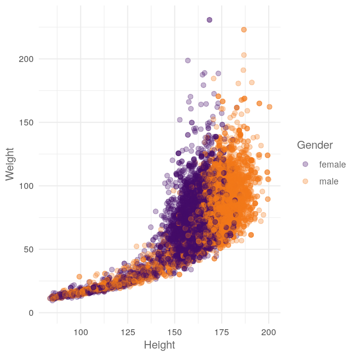
ggplot(NHANES, aes(x = Height, y = Weight, colour = Gender)) +
    geom_point(size = 2, alpha = 0.3) +
    scale_colour_viridis_d(option = "B", begin = 0.2, end = 0.7) +
    theme_minimal() +
    theme(text = element_text(colour = "grey40"))
#> Warning: Removed 366 rows containing missing values (geom_point).

Like before, maybe we want to see the scatter plot by different variables. So let’s get it into function form:

plot_scatter_by_group <- function() {
    scatter_plot <- ggplot(NHANES, aes(x = Height, y = Weight,
                                       colour = Gender)) +
        geom_point(size = 2, alpha = 0.3) +
        scale_colour_viridis_d(option = "B", begin = 0.2, end = 0.7) +
        theme_minimal() +
        theme(text = element_text(colour = "grey40"))
    return(scatter_plot)
}

Then let’s add in the arguments.

plot_scatter_by_group <- function(.dataset, .xvar, .yvar, .groupvar) {
    scatter_plot <- ggplot(.dataset, aes(x = .xvar, y = .yvar,
                                         colour = .groupvar)) +
        geom_point(size = 2, alpha = 0.3) +
        scale_colour_viridis_d(option = "B", begin = 0.2, end = 0.7) +
        theme_minimal() +
        theme(text = element_text(colour = "grey40"))
    return(scatter_plot)
}

Like the dplyr code above, this function won’t work because it also uses NSE, so ggplot2 will be confused by the x = .xvar since it will think you are asking for the .xvar column in the dataset. So, we need to change aes() to aes_string() to force ggplot2 to read .xvar as a character string that is the name of the column you want to plot.

plot_scatter_by_group <- function(.dataset, .xvar, .yvar, .groupvar) {
    scatter_plot <- ggplot(.dataset, aes_string(x = .xvar, y = .yvar,
                                                colour = .groupvar)) +
        geom_point(size = 2, alpha = 0.3) +
        scale_colour_viridis_d(option = "B", begin = 0.2, end = 0.7) +
        theme_minimal() +
        theme(text = element_text(colour = "grey40"))
    return(scatter_plot)
}
plot_scatter_by_group(NHANES, "Height", "Weight", "Gender")
#> Warning: Removed 366 rows containing missing values (geom_point).

Let’s add in the stopifnot, ggplot2:: explicit calls, and the roxygen documentation (Ctrl-Alt-Shift-R):

#' Create a scatter plot with colouring by categorical variable.
#'
#' @param .dataset Data to plot.
#' @param .xvar Variable for the x axis.
#' @param .yvar Variable for the y axis.
#' @param .groupvar The variable to group/color by.
#'
#' @return Creates a ggplot.
#'
plot_scatter_by_group <- function(.dataset, .xvar, .yvar, .groupvar) {
    stopifnot(is.character(.xvar), is.character(.yvar), is.character(.groupvar))
    scatter_plot <-
        ggplot2::ggplot(.dataset, ggplot2::aes_string(x = .xvar, y = .yvar,
                                                      colour = .groupvar)) +
        ggplot2::geom_point(size = 2, alpha = 0.3) +
        ggplot2::scale_colour_viridis_d(option = "B", begin = 0.2, end = 0.7) +
        ggplot2::theme_minimal() +
        ggplot2::theme(text = ggplot2::element_text(colour = "grey40"))
    return(scatter_plot)
}

Now we can do other plots easily:

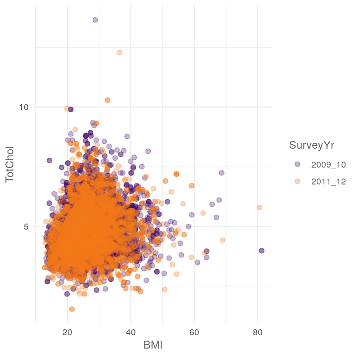
plot_scatter_by_group(NHANES, "BMI", "TotChol", "SurveyYr")
#> Warning: Removed 1594 rows containing missing values (geom_point).

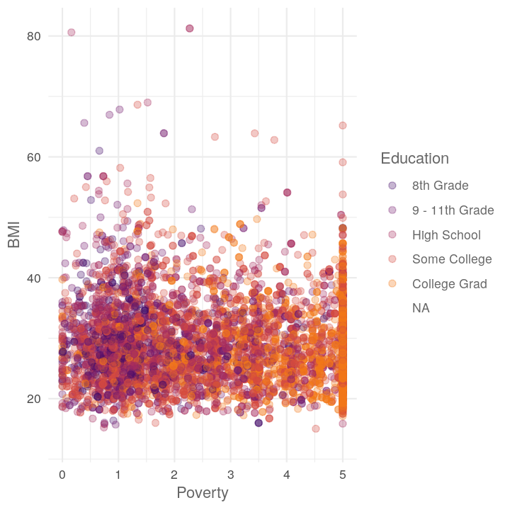
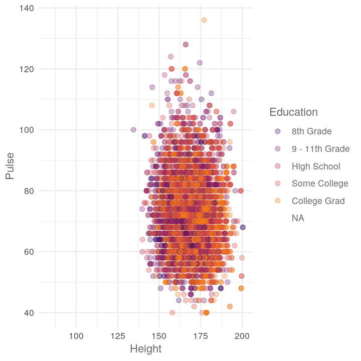
plot_scatter_by_group(NHANES, "Poverty", "BMI", "Education")
#> Warning: Removed 3368 rows containing missing values (geom_point).

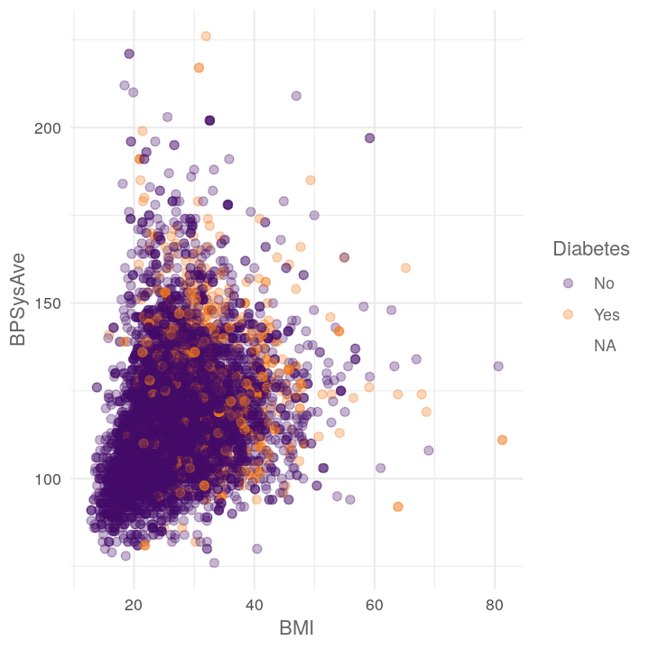
plot_scatter_by_group(NHANES, "BMI", "BPSysAve", "Diabetes")
#> Warning: Removed 1518 rows containing missing values (geom_point).

Iterating over items

You notice above that we copied and pasted multiple plot_scatter_by_group() calls to create three plots. Sometimes this is ok, but often when you start doing mostly the same thing, it’s better to try to reduce your repetition (i.e. don’t repeat yourself, DRY). Here we will get into iterations and using “functional programming” via the map function from the purrr package. Functional programming is a way of making use of vectors and vectorisation to “loop” over things (rather than use for loops). There are several reasons why you should avoid for loops in R.

They are computationally very slow and easily use a lot of RAM memory.
They are difficult to read and debug.
They aren’t very expressive, meaning they don’t state a higher “purpose”, just that they loop over something.

But functionals, like map and most functions inside purrr (or base R functions like lapply, sapply) let you ignore the tiny details and focus on doing your intent. You intend to sum a vector of numbers, not loop over each number and add to the total (as you would in a for loop).

For the example, let’s say we want to calculate the mean and SD for several categorical variables. We can use map to easily do this, by giving it a vector of variables and providing the function to apply to each:

map(c("SurveyYr", "Diabetes", "Gender"),
    # the ~ tells map the next code is all together as one argument
    # .x says to insert the value from the first argument of map (Diabetes, etc)
    ~mean_sd_by_group(NHANES, .x))
#> [[1]]
#> # A tibble: 5 x 3
#>   Measurement `2009_10`     `2011_12`
#>   <chr>       <chr>         <chr>
#> 1 BMI         26.88 (7.47)  26.44 (7.28)
#> 2 BPDiaAve    66.66 (14.22) 68.3 (14.45)
#> 3 BPSysAve    117.6 (17.09) 118.7 (17.39)
#> 4 Pulse       73.49 (12.17) 73.63 (12.14)
#> 5 TotChol     4.93 (1.08)   4.83 (1.07)
#>
#> [[2]]
#> # A tibble: 5 x 3
#>   Measurement No             Yes
#>   <chr>       <chr>          <chr>
#> 1 BMI         26.16 (7.09)   32.56 (8.15)
#> 2 BPDiaAve    67.43 (14.37)  68.04 (14.17)
#> 3 BPSysAve    117.23 (16.73) 127.95 (19.42)
#> 4 Pulse       73.58 (12.05)  73.32 (13.22)
#> 5 TotChol     4.89 (1.07)    4.78 (1.15)
#>
#> [[3]]
#> # A tibble: 5 x 3
#>   Measurement female         male
#>   <chr>       <chr>          <chr>
#> 1 BMI         26.77 (7.9)    26.55 (6.81)
#> 2 BPDiaAve    66.39 (13.5)   68.58 (15.09)
#> 3 BPSysAve    116.31 (17.82) 120.02 (16.45)
#> 4 Pulse       75.43 (11.93)  71.67 (12.1)
#> 5 TotChol     4.96 (1.08)    4.8 (1.07)

It seems deceptively simple but there is a massive amount of power from doing this sort of coding. Let’s try with the plots.

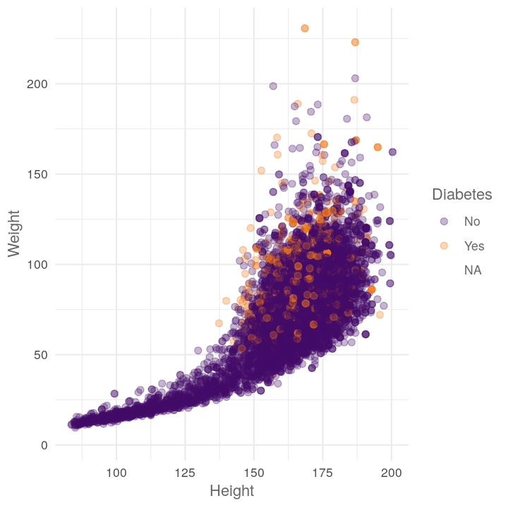
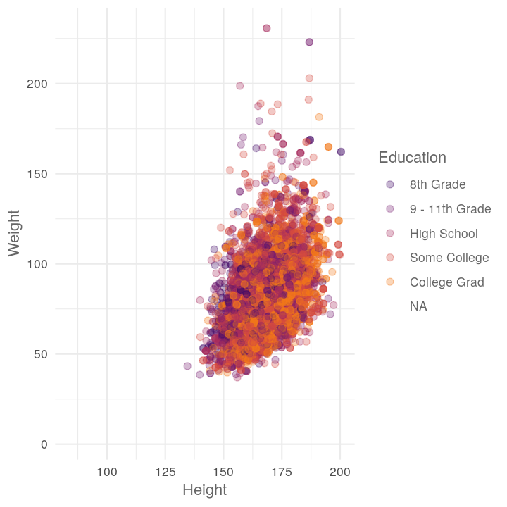
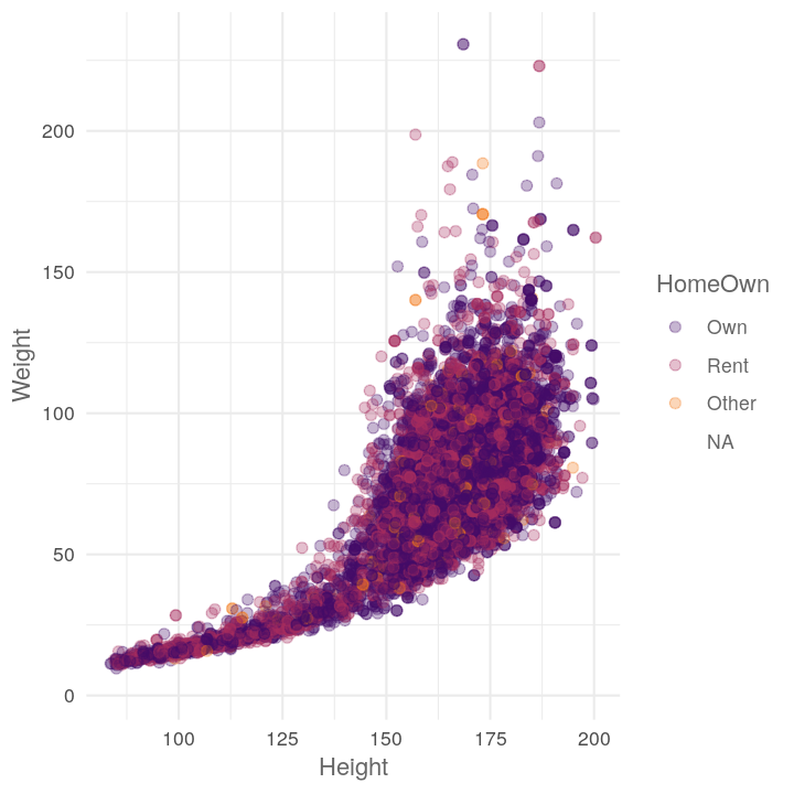
map(c("Diabetes", "Education", "HomeOwn"),
    ~plot_scatter_by_group(NHANES, "Height", "Weight", .x))
#> [[1]]
#> Warning: Removed 371 rows containing missing values (geom_point).

#>
#> [[2]]
#> Warning: Removed 2842 rows containing missing values (geom_point).

#>
#> [[3]]
#> Warning: Removed 426 rows containing missing values (geom_point).

What if we want to provide two things at once? We can use map2 for that! (Note, the two arguments should be the same length.)

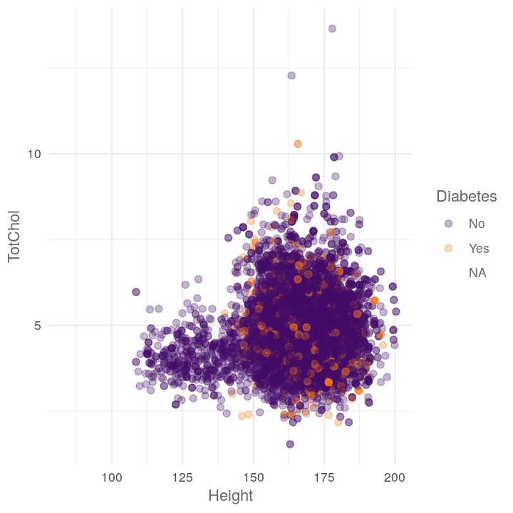
map2(c("TotChol", "Pulse"),
    c("Diabetes", "Education"),
    # .y is for the second argument of map
    ~plot_scatter_by_group(NHANES, "Height", .x, .y))
#> [[1]]
#> Warning: Removed 1587 rows containing missing values (geom_point).

#>
#> [[2]]
#> Warning: Removed 3072 rows containing missing values (geom_point).

If you want to do all combinations of two vectors, use the purrr function cross_df() to create a data.frame of the combinations. Note that, like most purrr functions, it takes a list as input.

all_combinations <- cross_df(list(
    xvar = c("TotChol", "Pulse"),
    groupvar = c("Diabetes", "Education")
    ))
all_combinations
#> # A tibble: 4 x 2
#>   xvar    groupvar
#>   <chr>   <chr>
#> 1 TotChol Diabetes
#> 2 Pulse   Diabetes
#> 3 TotChol Education
#> 4 Pulse   Education

map2(all_combinations$xvar, all_combinations$groupvar,
    ~plot_scatter_by_group(NHANES, "BMI", .x, .y))

Using map is really useful when importing raw data that is in a standard form and structure. Combined with the fs package (fs for filesystem), this is very powerful. To show how to do it, let’s first export NHANES into the data/ folder.

NHANES %>%
    filter(SurveyYr == "2009_10") %>%
    write_csv(here::here("data/nhanes-2009_10.csv"))

NHANES %>%
    filter(SurveyYr == "2011_12") %>%
    write_csv(here::here("data/nhanes-2011_12.csv"))

Then we can use the dir_ls() (for directory list) from fs combined with the regexp (for regular expression) argument to show all files that have nhanes in the name, have anything in the middle (.*), and end with ($) csv.

data_files <- fs::dir_ls(here::here("data/"), regexp = "nhanes-.*csv$")
data_files
#> /home/luke/Documents/teaching/dda-rcourse/data/nhanes-2009_10.csv
#> /home/luke/Documents/teaching/dda-rcourse/data/nhanes-2011_12.csv

Then we can import all at once using map_dfr (for map and convert to a df data.frame, stacking by r row):

data_files %>%
    map_dfr(read_csv)
#> Parsed with column specification:
#> cols(
#>   .default = col_double(),
#>   SurveyYr = col_character(),
#>   Gender = col_character(),
#>   AgeDecade = col_character(),
#>   Race1 = col_character(),
#>   Race3 = col_logical(),
#>   Education = col_character(),
#>   MaritalStatus = col_character(),
#>   HHIncome = col_character(),
#>   HomeOwn = col_character(),
#>   Work = col_character(),
#>   BMICatUnder20yrs = col_logical(),
#>   BMI_WHO = col_character(),
#>   Testosterone = col_logical(),
#>   Diabetes = col_character(),
#>   HealthGen = col_character(),
#>   LittleInterest = col_character(),
#>   Depressed = col_character(),
#>   SleepTrouble = col_character(),
#>   PhysActive = col_character(),
#>   TVHrsDay = col_logical()
#>   # ... with 12 more columns
#> )
#> See spec(...) for full column specifications.
#> Parsed with column specification:
#> cols(
#>   .default = col_double(),
#>   SurveyYr = col_character(),
#>   Gender = col_character(),
#>   AgeDecade = col_character(),
#>   Race1 = col_character(),
#>   Race3 = col_character(),
#>   Education = col_character(),
#>   MaritalStatus = col_character(),
#>   HHIncome = col_character(),
#>   HomeOwn = col_character(),
#>   Work = col_character(),
#>   BMICatUnder20yrs = col_character(),
#>   BMI_WHO = col_character(),
#>   Diabetes = col_character(),
#>   HealthGen = col_character(),
#>   LittleInterest = col_character(),
#>   Depressed = col_character(),
#>   SleepTrouble = col_character(),
#>   PhysActive = col_character(),
#>   TVHrsDay = col_character(),
#>   CompHrsDay = col_character()
#>   # ... with 13 more columns
#> )
#> See spec(...) for full column specifications.
#> # A tibble: 10,000 x 76
#>       ID SurveyYr Gender   Age AgeDecade AgeMonths Race1 Race3 Education
#>    <dbl> <chr>    <chr>  <dbl> <chr>         <dbl> <chr> <chr> <chr>
#>  1 51624 2009_10  male      34 30-39           409 White <NA>  High Sch…
#>  2 51624 2009_10  male      34 30-39           409 White <NA>  High Sch…
#>  3 51624 2009_10  male      34 30-39           409 White <NA>  High Sch…
#>  4 51625 2009_10  male       4 0-9              49 Other <NA>  <NA>
#>  5 51630 2009_10  female    49 40-49           596 White <NA>  Some Col…
#>  6 51638 2009_10  male       9 0-9             115 White <NA>  <NA>
#>  7 51646 2009_10  male       8 0-9             101 White <NA>  <NA>
#>  8 51647 2009_10  female    45 40-49           541 White <NA>  College …
#>  9 51647 2009_10  female    45 40-49           541 White <NA>  College …
#> 10 51647 2009_10  female    45 40-49           541 White <NA>  College …
#> # … with 9,990 more rows, and 67 more variables: MaritalStatus <chr>,
#> #   HHIncome <chr>, HHIncomeMid <dbl>, Poverty <dbl>, HomeRooms <dbl>,
#> #   HomeOwn <chr>, Work <chr>, Weight <dbl>, Length <dbl>, HeadCirc <dbl>,
#> #   Height <dbl>, BMI <dbl>, BMICatUnder20yrs <chr>, BMI_WHO <chr>,
#> #   Pulse <dbl>, BPSysAve <dbl>, BPDiaAve <dbl>, BPSys1 <dbl>,
#> #   BPDia1 <dbl>, BPSys2 <dbl>, BPDia2 <dbl>, BPSys3 <dbl>, BPDia3 <dbl>,
#> #   Testosterone <dbl>, DirectChol <dbl>, TotChol <dbl>, UrineVol1 <dbl>,
#> #   UrineFlow1 <dbl>, UrineVol2 <dbl>, UrineFlow2 <dbl>, Diabetes <chr>,
#> #   DiabetesAge <dbl>, HealthGen <chr>, DaysPhysHlthBad <dbl>,
#> #   DaysMentHlthBad <dbl>, LittleInterest <chr>, Depressed <chr>,
#> #   nPregnancies <dbl>, nBabies <dbl>, Age1stBaby <dbl>,
#> #   SleepHrsNight <dbl>, SleepTrouble <chr>, PhysActive <chr>,
#> #   PhysActiveDays <dbl>, TVHrsDay <chr>, CompHrsDay <chr>,
#> #   TVHrsDayChild <dbl>, CompHrsDayChild <dbl>, Alcohol12PlusYr <chr>,
#> #   AlcoholDay <dbl>, AlcoholYear <dbl>, SmokeNow <chr>, Smoke100 <chr>,
#> #   Smoke100n <chr>, SmokeAge <dbl>, Marijuana <chr>, AgeFirstMarij <dbl>,
#> #   RegularMarij <chr>, AgeRegMarij <dbl>, HardDrugs <chr>, SexEver <chr>,
#> #   SexAge <dbl>, SexNumPartnLife <dbl>, SexNumPartYear <dbl>,
#> #   SameSex <chr>, SexOrientation <chr>, PregnantNow <chr>

Nifty eh?

Easier to use parallel processing with map

One big reason to get comfortable and good at using map is because you can use parallel processing to speed up your analysis with the future_ series of functions from the furrr package.

library(furrr)
# Use a combination of more of your CPU or creating multiple R sessions
plan(multiprocess)

# Use parallel processing
future_map2(all_combinations$xvar, all_combinations$groupvar,
    ~plot_scatter_by_group(NHANES, "BMI", .x, .y))

Final exercise

Time: Until end of session.

Create a new file for this exercise:

usethis::use_r("efficiency-exercise")

Copy and paste the template code (further below) into the R/efficiency-exercise.R file. Simplify the below code into three functions. Then iterate with one map to read in and wrangle each dataset, followed by two map calls to create the two different plots for each dataset.

nhanes_2009 <- read_csv(here::here("data/nhanes-2009_10.csv"))

nhanes_2009 %>%
    mutate(ProblemBMIs = !between(BMI, 18.5, 40)) %>%
    filter(!is.na(ProblemBMIs)) %>%
    select(Age, Poverty, Pulse, BPSysAve, BPDiaAve, TotChol,
           SleepHrsNight, PhysActiveDays, ProblemBMIs) %>%
    gather(Measurement, Value, -ProblemBMIs) %>%
    na.omit() %>%
    ggplot(aes(y = Value, x = Measurement, colour = ProblemBMIs)) +
    geom_jitter(position = position_dodge(width = 0.6)) +
    scale_color_viridis_d(end = 0.8) +
    labs(y = "", x = "") +
    theme_minimal() +
    theme(legend.position = c(0.85, 0.85)) +
    coord_flip()

nhanes_2009 %>%
    mutate(ProblemBMIs = !between(BMI, 18.5, 40)) %>%
    filter(!is.na(ProblemBMIs)) %>%
    select(Age, Poverty, Pulse, BPSysAve, BPDiaAve, TotChol,
           SleepHrsNight, PhysActiveDays, ProblemBMIs) %>%
    gather(Measurement, Value, -ProblemBMIs) %>%
    na.omit() %>%
    ggplot(aes(x = Value, fill = ProblemBMIs)) +
    geom_density(alpha = 0.35) +
    facet_wrap(~Measurement, scales = "free") +
    scale_fill_viridis_d(end = 0.8) +
    labs(y = "", x = "") +
    theme_minimal() +
    theme(legend.position = c(0.85, 0.15),
          strip.text = element_text(face = "bold"))

nhanes_2011 <- read_csv(here::here("data/nhanes-2011_12.csv"))

nhanes_2011 %>%
    mutate(ProblemBMIs = !between(BMI, 18.5, 40)) %>%
    filter(!is.na(ProblemBMIs)) %>%
    select(Age, Poverty, Pulse, BPSysAve, BPDiaAve, TotChol,
           SleepHrsNight, PhysActiveDays, ProblemBMIs) %>%
    gather(Measurement, Value, -ProblemBMIs) %>%
    na.omit() %>%
    ggplot(aes(y = Value, x = Measurement, colour = ProblemBMIs)) +
    geom_jitter(position = position_dodge(width = 0.6)) +
    scale_color_viridis_d(end = 0.8) +
    labs(y = "", x = "") +
    theme_minimal() +
    theme(legend.position = c(0.85, 0.85)) +
    coord_flip()

nhanes_2011 %>%
    mutate(ProblemBMIs = !between(BMI, 18.5, 40)) %>%
    filter(!is.na(ProblemBMIs)) %>%
    select(Age, Poverty, Pulse, BPSysAve, BPDiaAve, TotChol,
           SleepHrsNight, PhysActiveDays, ProblemBMIs) %>%
    gather(Measurement, Value, -ProblemBMIs) %>%
    na.omit() %>%
    ggplot(aes(x = Value, fill = ProblemBMIs)) +
    geom_density(alpha = 0.35) +
    facet_wrap(~Measurement, scales = "free") +
    scale_fill_viridis_d(end = 0.8) +
    labs(y = "", x = "") +
    theme_minimal() +
    theme(legend.position = c(0.85, 0.15),
          strip.text = element_text(face = "bold"))

Use this as a template for completing the exercise:

read_mutate_gather <- function(.file_path) {
    .file_path %>%
        ___
}

plot_jitter <- function(.dataset) {
    .dataset %>%
        ___
}

plot_density <- function(.dataset) {
    .dataset %>%
        ___
}

# Read in and wrangle each csv file
data_list <-
    c(here::here("data/nhanes-2009_10.csv"),
      here::here("data/nhanes-2011_12.csv")) %>%
    # (keep as list, i.e. don't use map_dfr)
    ___(___)

# Plot each data with jitters
___(data_list, ___)

# Plot each data with density
___(data_list, ___)

If you’ve finished the exercise early, true using the furrr package to implement parallel processing on these map calls.

Resources for learning and help

For learning:

Efficient R Programming (online and free book)
Functions chapter in R for Data Science book
map section in the R for Data Science book.
R/ chapter in R Packages book (online and free).
Documenting functions chapter in R Packages book.
Functions in R DataCamp course (need subscription).
Working with map and the purrr package DataCamp course (need subscription)
Very advanced (for those interested) details about functions from Advanced R book (again, online and free).
Follow the principles of tidy tools when making functions.

For help:

Last updated on Mar 11, 2019