Session details
Objectives
- To become aware of the importance of reproducibility of data analyses, for your own productivity and for greater rigor in science.
- To create reproducible documents interwoven with R code that can be easily updated by changing the code or data.
- To know where to go for continued learning.
At the end of this session you will be able:
- Write text, headers, citations, and other writing tasks in RStudio using Markdown.
- Insert R code chunks in the Markdown document that will create figures, tables, and/or numbers.
- As part of the assignment, you will create an analytically reproducible document showing your analysis code and output.
Why try to be reproducible?
Well, first of all, reproducibility and replicability are cornerstones of doing rigorous and sound science. As we’ve learned, reproducibility in science is lacking. Being reproducible isn’t just doing better science, it can also:
- Make you much more efficient and productive, as less time is spent between coding and putting your results in the document.
- Make you more confident in your results, as what you report and show as figures or tables will be exactly what you get from your analysis. No copying and pasting required!
- It’s actually a lot of fun! 😉
Hopefully by the end of this session you’ll try to start using R Markdown files for writing your manuscripts and other technical documents. Believe us, it can save soooo much time in the end, after you’ve learned how to incorporate text with R code, and make your analysis and work more reproducible. Plus you can create some beautifully formatting reports, waaayyyy more easily than you can if you did it all in Word. As a bonus, switching between citation formats for different journals is a breeze.
Markdown syntax
First, let’s create and save an R Markdown file. Go to File -> New File -> R
Markdown and a dialog box will pop up. Type in Reproducible documents in the
title section and your name in the author section. Choose the HTML output format.
Save this file as rmarkdown-session.Rmd in the doc/ folder.
Markdown is a markup syntax and formatting tool that allows you write in plain text (like R code and scripts) a document that can convert to a vast range of other document types (e.g. HTML, PDF, Word documents, slides, posters, websites). In fact, this website is built from R and Markdown! (Plus many other things, like HTML.) The Markdown used in R Markdown is based on pandoc, a very powerful and well-maintained software tool for document conversion. Text formatting is done using special characters (like commands) to indicate what is bolded, a header, a list, and so on. Most features needed for writing a scientific document are available in Markdown, but not all. My suggestion is to try to fit your writing around Markdown, rather than force or fight Markdown to do something it wasn’t designed to do. You can do a lot with what Markdown has.
Headers
Creating headers (like chapters or sections) is indicated by one or more #:
# Header 1
Paragraph.
## Header 2
Paragraph.
### Header 3
Paragraph.
Text formatting
**bold**gives bold.*italics*gives italics.super^script^gives super^script^.sub~script~gives sub~script~.
Lists
Unnumbered list:
- item 1
- item 2
- item 3
gives…
- item 1
- item 2
- item 3
Numbered list:
1. item 1
2. item 2
3. item 3
gives…
- item 1
- item 2
- item 3
Block quotes
One can also create quotes:
> Block quote
gives…
Block quote
Adding footnotes
Footnotes can be done using the following command:
Footnote[^1]
[^1]: Footnote content
gives…
Footnote1
Inserting pictures
A png, jpeg, or pdf image can be attached by doing (here, use an image of your own):
gives…

Note: Can also include links to images from the Internet, as a URL link.
Adding links to websites
And a link can be linked in the following format:
[Link](https://google.com)
gives…
Inserting (simple) tables
You can insert tables using Markdown too. I wouldn’t recommend doing it for complicated tables though, as it can get tedious fast! (My recommended approach for more complex or bigger tables is to make a data frame in R and then use create the table as shown in the section below.)
| | Fun | Serious |
|:--|----:|--------:|
| **Happy** | 1234 | 5678 |
| **Sad** | 123 | 456 |
gives…
| Fun | Serious | |
|---|---|---|
| Happy | 1234 | 5678 |
| Sad | 123 | 456 |
The |---:| or |:---| tell the table to left-align or right-align the values
in the column. Center-align is |:----:|.
Break time.
R Markdown
R Markdown is an extension of Markdown that combines R code and Markdown formatting markup. Output from R code gets inserted into the document for a seamless integration of document writing and analysis.
YAML header/metadata
Most Markdown documents (especially for R Markdown) include YAML metadata at
the top of the document, surrounded by --- on the top and bottom. The YAML
contains metadata and options for the entire document. For instance, the title
or author but also the output format you want to use, such as Word, HTML, or PDF
(if you want to create a beautiful PDF, you need to install the R package
tinytex). There are many more output formats, but these are the most common.
---
title: "Document title"
author: Your Name
output: word_document
---
There are additional options you can set in the output field, which we will show later below.
Now the best part! Inserting R code
One of the most powerful and useful features of R Markdown is its ability to
combine text and R code in the same document! You can insert plots by including a
code chunk, like the one below. The options added to the code chunk tell it to
add a caption, to set the height and width of the figure, and to prevent the code
chunk from showing up in the final document (echo=FALSE). The bmi-plot label is
the name of the code chunk (which you can see in the “Document Outline”, found
using Ctrl-Shift-O, if you have the options set in the Tools -> Global
Options -> R Markdown).
NOTE: Code chunk labels should be named without _, spaces, or . and
instead should be one word or be separated by -. While an error may not
necessarily occur, there can be some unintended side effects that will cause you
some annoyance without knowing the reason.
```{r bmi-plot, fig.cap="Add your figure title here.", fig.height=8, fig.width=8, echo=FALSE}
ggplot(NHANES, aes(x = Height, fill = Gender)) +
geom_density(alpha = 0.4) +
scale_fill_brewer(type = "qual", palette = "Dark2") +
theme_minimal() +
theme(legend.position = c(0.2, 0.85))
```
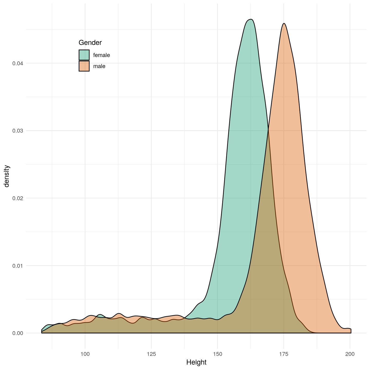
Figure 1 Add your figure title here.
You can also create tables by using the kable() function from the knitr package:
```{r mean-bmi-table, echo=FALSE}
library(knitr)
NHANES %>%
select(SurveyYr, BMI, Diabetes) %>%
group_by(SurveyYr, Diabetes) %>%
summarise(MeanBMI = mean(BMI, na.rm = TRUE)) %>%
spread(SurveyYr, MeanBMI) %>%
kable(caption = "Table caption here")
```
| Diabetes | 2009_10 | 2011_12 |
|---|---|---|
| No | 26.38 | 25.95 |
| Yes | 32.59 | 32.53 |
| (Missing) | 40.76 | 22.20 |
Or just print out a number to the document:
```{r, echo=FALSE}
cor(NHANES$Height, NHANES$Weight)
```
#> [1] -0.1175698
Inline R code
You can also include R code within the text. You can use this to directly insert numbers into the text of the document. By using something like:
The mean of BMI is `r round(mean(NHANES$BMI, na.rm = TRUE), 2)`.
Gives…
The mean of BMI is 26.66.
Note: Inline R code can only insert a single number or character value, nothing more.
Other features
Citing literature with R Markdown
If you want to insert a citation use [@Hoejsgaard2006a], which will look like
(Højsgaard, Halekoh, and Yan, 2006), and the reference is then inserted onto
the bottom of the document. You need to add a line to the YAML header like this:
---
title: "My report"
author: "Me!"
bibliography: my_references.bib
---
Make sure to add this to the end of your file:
# References
Making your report prettier
This part mostly applies to HTML-based and PDF2 outputs, since programmatically modifying or setting templates Word documents is rather difficult3. Changing broad features of a document can be done by setting the “theme” of the document. Add an option in the YAML metadata like:
---
title: "My report"
output:
html_document:
theme: sandstone
---
Check out the R Markdown documentation for more types of themes you can use for HTML documents, and advanced topics such as parameterized R Markdown documents. Most of the Bootswatch themes are available for use in R Markdown to HTML conversion.
Final exercise: Starting creating the assignment report
Time: Until the end of the session.
Open RStudio and create an R Markdown document:
File -> New File -> R
Markdown
Save the file in doc/ and name the file assignment.Rmd. In the R Markdown
document, include the following “Header 1” # sections:
- Abstract
- Introduction
- Material and Methods
- Results
- Discussion
- Conclusion
(You don’t have to actually fill these out for the assignment.) Compile it by
pressing the icon Knit to HTML or by typing Ctrl-Shift-K. Then:
- Write some random words below the Abstract section, while using bold and italics.
- Include an unnumbered list below Introduction listing two or three fake objectives.
- Include a “Header 2” (
##) called “Statistical analysis” below “Material and Methods”.
Compile (“knit”) the document again and see what happens. Then, add these additional features to the document:
- Include a random picture with caption (of your research or of any png you find in your PC).
- Include a footnote.
- Include the link of your GitHub (if you created one) or of your academic profile.
Then, add some R code chunks with code to wrangle your data and also to create a figure (you can copy and paste from previous sessions). Include these code chunks in the “Results” section. During the group work sessions, you can use this as a template for the assignment.
Resources for learning and help
For learning:
- RStudio tutorial on using R Markdown
- Markdown syntax guide
- Online book for R Markdown
- Pandoc Markdown Manual (R Markdown uses pandoc)
- R for Data Science
For help:
- RStudio helpful cheatsheets
- R Markdown cheatsheet (downloads a pdf file)
- R Markdown reference cheatsheet
Acknowledgements
Parts of this lesson were modified from the UofTCoders R Course and from a session taught at the Aarhus University Open Coders, with contributions from Maria Izabel Cavassim Alves (@izabelcavassim), PhD student at AU in Bioinformatics.
References
Include this header to list the bibliography.
- Footnote content ^
- Knitting to PDF will require that you install LaTeX using the tinytex R package. After you install LaTeX you can create truly beautifully typeset PDF documents. ^
- If you really want to do it, the best way is to create your template in the
.odt, and then convert to.docx. Here is a good place to start. ^